Lead engineers are expected to understand the following:
How to calculate activation time for a water-based suppression head from a stead-state (pool) fire.
How to calculate activation time from a transient fire using an Euler's approach (DETACT).
How to use the Hazen Williams formula and understand the basics of expected pressure losses for a design area.
How to read an HRR graph and know sources (NFRL/NIST) where to find fire profiles.
Understand density requirements from NFPA 13 for various protection categories.
How to find the correct version of NFPA 13 for your application.
How to determine the pressure and flow for a given head or system.
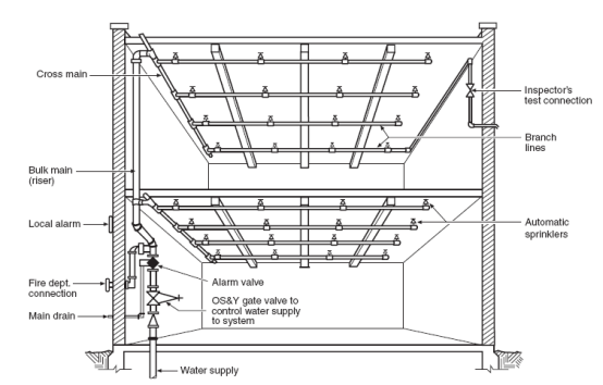
There are standard operational definitions used by our program that need to be understood when communicating information. The following image shows basic information
for a suppression system.
Figure 1: Nomenclature for suppression systems.
It is important to understand that water supply availability to the Base Of the Riser (BOR) defines a threshold for system performance. This water goes through the
riser, the bulk main, the cross main and the branch lines to reach the sprinkler head. The frictional losses associated with this transportion result in pressure losses that
affect the amount of water available at the sprinkler head. Furthermore, the protected items where the head is located need to have adequate water to protect the type
of material that is threatened by fire.
Figure 2: How water quantity affects fire control.
Figure 2 demonstrates the sensativity to fire growth as a function of water quantity. Understanding the type of commodity or combustible loading in an area
will impact how the suppression system is designed regarding density and expected area of protection. Misunderstanding this topic will result in too little
water that will not adequately control the fire, or too much water that unnecessarily increases the overall system cost.
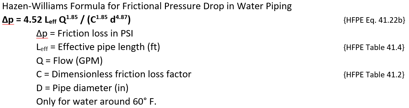
Figure 3: Hazen William Equation.
The Hazen Williams equation shown in Figure 3 is typically good until around 25 ft/s. The Code does not specify that velocity value, but discretion needs to be
applied as the velocity increases. Your design may benefit by examining the results from both the Hazen Williams and the Darci Weisbach equation as the velocity
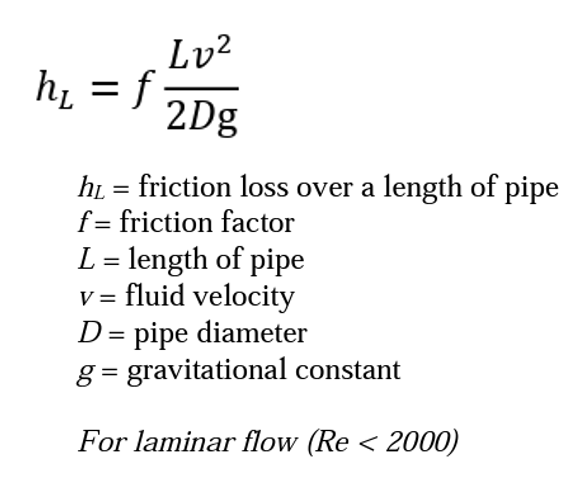
approaches 25 ft/s. The Darci Weisbach equation is shown in Figure 4. Use the Moody chart for the "f" frictional factor. You will need to calculate the Reynold's number (Re)
to find the "f" value. A "C" value of 120 is typically acceptable for new installations for typical situations. See the NFPA FPH or SFPE HFPE suppression sections
for corrosive water or MIC concerns. Such issues will result in a lower "C" value.
Figure 4: Darci Weisbach equation.
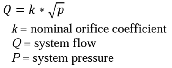
General water flow can be calculated if the "K" factor of an orifice is known and if the pressure is also measured. The equation for calculating the sprinkler flow using the
sprinkler K-factor is shown in Figure 5. The K-factor is provided by the factory for sprinkler heads, but can also be calculated if the flow rate and pressure of a system
is known. A 1/2" sprinkler orifice is equivalent to a K-factor of 5.6.
Figure 5: Flow equation.
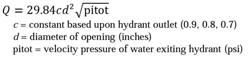
A lead engineer frequently oversees personnel performing hydrant flow tests. The equation for calculating flow from when the pressure is known and the geometry of the
hydrant is characterized is shown in Figure 6. The lead engineer should also understand how to calculate flow for other pressures given the flow and pressure characteristics
of a given hydrant. Additional information for this is found in SFPE HFPE Chapter 41.
Figure 6: Hydrant flow test equation.
Generally, it is important for the lead engineering to know that the pressure due to elevation is simple to calculate. Pressure (PSI) is equal to 0.433 multipled by the
height in ft. After performing the various calculations for water flow, the lead engineer needs to understand if the suppression system meets performance expectation for both
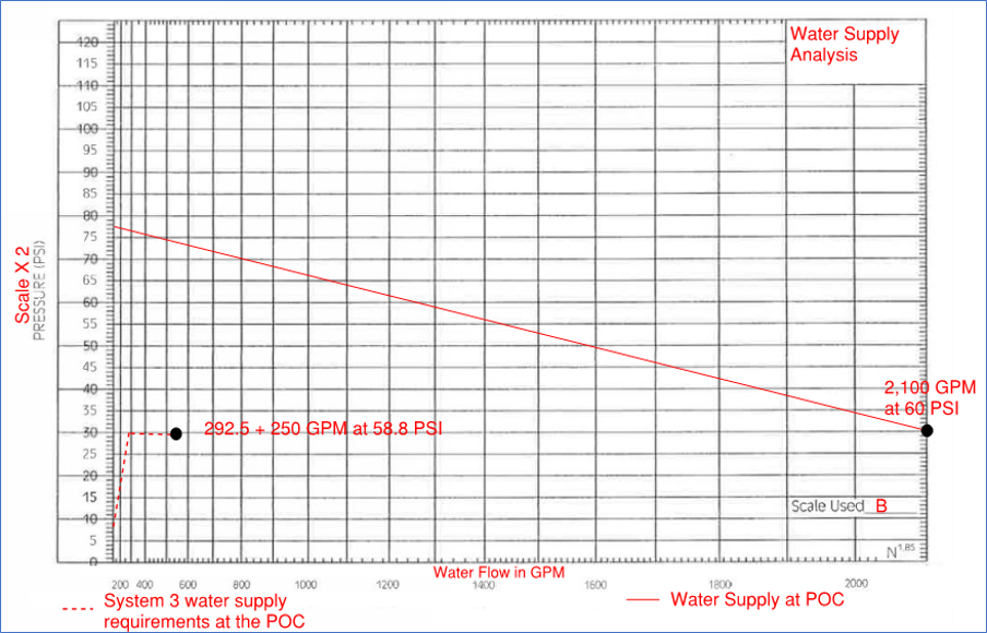
the available water and for the type of system necessary. Figure 7 shows a waterflow graph that identifies that enough water is available at the base of the riser.
Because of the "4.87" power for the diameter in the deonominator of the Hazen Williams equation, small decreases in the diameter result in significant changes
in frictional losses. Similarly, the "1.85" power for flow (Q) in the numerator also demonstrates a significant increase in pressure as flow increases. These two
powers need to be understood when characterizing a system. Proper measurements need to be made for the piping size. Accurate inside diameters of the piping schedule
need to be looked up instead of nominal values. Figure 7 shows an example from a program building where ample water supply is available. This graph proves
that the system is acceptable. A lead engineer is expected to understand the basic principles in this figure.
Figure 7: Basic water supply graph.
Frequently, scenarios exist where the lead engineer is required to estimate sprinkler performance as a function of a combustible loading. This involves calculating
an estimated HRR using either real NIST calorimetry data or by using one of several equations that define fires using the heat of combustion values for the materials.
A pool fire is a simple example of a stead-state HRR source. For instance, gasoline typically burns at a rate of 0.055 kg/s-m2, with a heat of combustion
at 43.7 MJ/kg. Knowing the area of a fire, the HRR can be calculated. The SFPE HFPE has specific sections that give the formulas and properties to use. The time for
sprinkler activation relies on the Response Time Index (RTI), the velocity of the gasses passing by the sprinkler head (u), the rated temperature of the detector (TD),
the temperature of the hot gasses (Tg), and the ambient temperature of the air (Ta). Figure 8 shows the typical formula used when a steady state fire
is affecting the suppression system. NFPA 13 provides a range for the RTI depending on whether a head is an SR or QR.
Figure 8: Stead-state suppression activation.
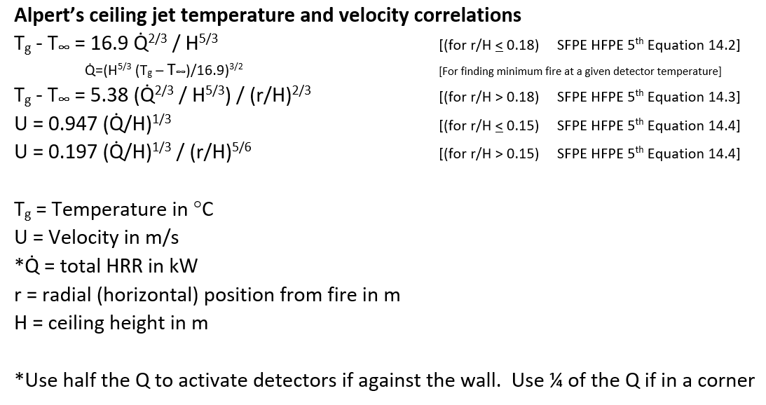
The velocity and temperature of the hot gasses going by a sprinkler head can be calculated from Alpert's ceiling jet equations found in Chapter 14 of the SFPE HFPE. The applicable
equations for the equation in Figure 8 are shown in Figure 9.
Figure 9: Alpert's Correlations.
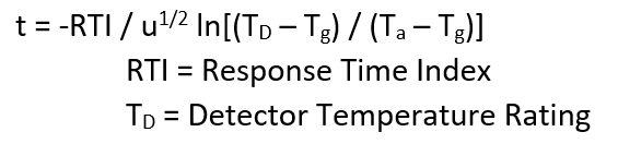
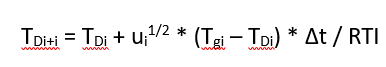
For transient fires, the gas velocity and temperature values can be calculated from Alpert's correlations on a time step basis using HRR as the input. These U and Tg
values can be used as inputs into the transient detector temperature equation shown in Figure 10. The "i" index simply represents a time step. Activation occures
when Tdi+1 reaches the rated detector temperature. This process can be done in an Excel spreadsheet using a time step typically at 1 second. This is an
Euler's numerical integration approach, and this process is known as the DETACT method, which is short for Detector Activation.
Figure 10: DETACT formula.
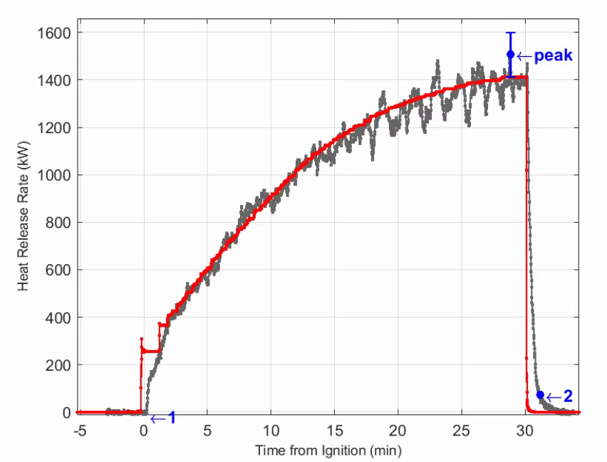
The HRR data for a transient fire can be obtained through calculations such as a "T"-squared model, or through actual recorded calorimetry data as available from
NIST. Figure 11
shows data from a kitchen fire. NIST has collected several applicable fire tests to model scenarios that we may encounter. The SFPE HFPE also has several
graphs of HRR. A helpful tool for digitizing graphed data is a web-plot digitizer. The HRR information can be calculated or extracted
and placed into Excel for input into the Alpert correlations.
Figure 11: NIST HRR data.
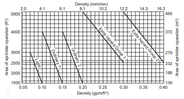
General code knowledge is required to be a lead engineer. An understanding of NFPA 13 regarding applicable density and area for the suppression design is required.
Situations arise where personnel may use an office area, conference room or other occupancy type as a temporary storage area elevating the suppression requirements
to meet the commodity classification specified for the type of miscellaneous storage occurring. NFPA 13 has specific definitions for such storage and has
requirements for water density that need to be validated if such storage is permitted. For instance, if a Class IV commodity is being stored in an area for
the IT group, where the area was formerly used as a cafeteria break room, and the area had an OH1 system, will the existing suppression system be
suitable for the new use, even if it is temporary? The control mode density curves are shown in Figure 12. The lead engineer is expected to understand
what this graph represents.
Figure 12: Control mode density curve.
Typically, the State adopted International Fire Code (IFC) is used as the applicable code. The IFC is frequently modified by the State. Chapter 80 of the IFC
has a list of references with the applicable versions to use. Frequently, these versions are modified by the State to different publication years. For instance,
the State of Idaho adopts the 2018 version of the IFC, but modifies Chapter 80 to specify the 2019 versions of NFPA 13 and 72. Reading the IFC by itself will
not show this modification. It is important to identify from the State what ammendments have been made. Another example from Idaho is where Appendices B-F have
been adopted from the IFC. Normally, appendices are not required. It is important to know such ammendments have been made as Appendix B and Appendix D have
specific requirements for water supplies and hydrant locations that would otherwise not be recognized.
A lead engineer will need to validate that adequate suppression is available when performing a plans review or judging whether a change of occupancy is acceptable,
such as when an area is used for miscellaneous storage. Most situations for new and modified designs, a software system such as HASS will be used to perform
hydraulic calculations and provide a convenient summary. Occasionally, a design area/density will need further analysis and will need hand calculations.
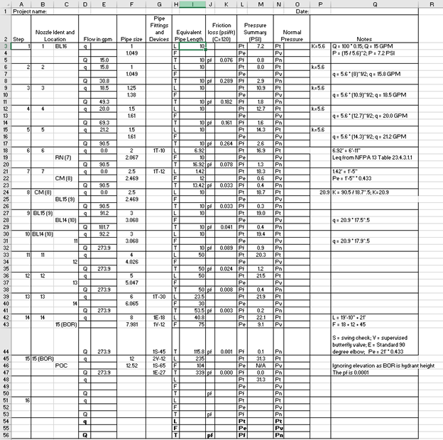
The lead engineer is expected to understand the basics of hand hydraulic calculations such as understanding equivalent length, elevation pressure, frictional pressure
losses, and how to calculate a K-factor for a branch line or system. It is important to have a basic understanding of how these calculations are used in a
design such as what is shown in Figure 13. This is an example of hydraulic calcuations for an OH1 system to validate that adequate flow was available from a riser.
Figure 13: Hydraulic calculations.